Finding coefficients of a polynomial
Part 1. Basic approach ("exact fit")
We need a table of n+1 values of the variables x and y in order to find the coefficients of an nth degree polynomial, P(x) = y.
Example.
We are looking for a third degree polynomial, P(x) = a1 + a2*x + a3*x2 + a4*x3, where a1, a2, a3, and a4 are unknown, and y = P(x). We have this table of four values of x and y,
| x: | -2 | -1 | 1 | 3 |
| y: | -5.8 | .9 | 1.1 | -12.3 |
To see these points on our TI-83/84 screen, make lists X and Y:
{-2, -1, 1, 3}→X
{-5.8, .9, 1.1, -12.3}→Y
Now go to STAT PLOT and turn Plot1 On. For Xlist enter X, and for Ylist enter Y. Choose the first mark, a little square.
Set WINDOW
Xmin=-5
Xmax=10
Ymin=-20
Ymax=30
Now press Graph and you will see

We want to put a 3rd degree polynomial through these 4 points.
We need to solve the following four equations in four unknowns, giving us values for the four coefficients, a1, a2, a3, and a4:
1*a1 + -2*a2 + (-2)2*a3 + (-2)3*a4 = -5.8
1*a1 + -1*a2 + (-1)2*a3 + (-1)3*a4 = .9
1*a1 + 1*a2 + 12*a3 + 13*a4 = 1.1
1*a1 + 3*a2 + 32*a3 + 33*a4 = -12.3
In matrix notation,
[C] * [X] = [D], or
[[1 -2 (-2)2 (-2)3] [[a1] [[-5.8]
[1 -1 (-1)2 (-1)3] * [a2] = [.9]
[1 1 12 13] [a3] [1.1]
[1 3 32 33] ] [a4] ] [-12.3]]
Store the square matrix in the 4 by 4 matrix variable [C], and store the matrix of y values in the 4 by 1 matrix [D], using the matrix editor.
From the home screen execute,
[C]-1[D]→[A] ENTER
The matrix [A] holds the coefficients a1, a2, a3, and a4 that we were looking for.
[A] = [[ 3]
[0]
[-2]
[ .1]]
So the polynomial is y = 3 -2x2 + .1x3.
You may check it. You already formed the two lists LX and LY above by setting
{-2, -1, 1, 3}→X and
{-5.8, .9, 1.1, -12.3}→Y.
Now under \Y= enter
\Y1=3 – 2X2 + .1X3
Now on the home screen enter
Y1(LX)-LY
You should see {0 0 0 0}
To see how the polynomial fits the four points, activate Y1 and Plot1, and GRAPH:

The polynomial nicely goes through all 4 points.
Part 2. Procedure for “best fit”
Now suppose we have a table of n+2 values of the variables x and y, and we want to find the coefficients of an nth degree polynomial. We show the procedure using an example.
Example.
We are looking for a third degree polynomial, P(x) = a1 + a2*x + a3*x2 + a4*x3, where a1, a2, a3, and a4 are unknown, and y = P(x). We have this table of five values of x and y,
| x: | -2 | -1 | 1 | 3 | 6 |
| y: | -5.8 | .9 | 1.1 | -12.3 | 4 |
Update the lists X and Y as follows:
{-2, -1, 1, 3, 6}→X
{-5.8, .9, 1.1, -12.3, 4}→Y
You can see these by graphing Plot1. Here is what the points look like on the screen:

We have the following five equations in four unknowns.
1*a1 + -2*a2 + (-2)2*a3 + (-2)3*a4 = -5.8
1*a1 + -1*a2 + (-1)2*a3 + (-1)3*a4 = .9
1*a1 + 1*a2 + 12*a3 + 13*a4 = 1.1
1*a1 + 3*a2 + 32*a3 + 33*a4 = -12.3
1*a1 + 6*a2 + 62*a3 + 63*a4 = 4
In general, we cannot find an exact solution, but we may try to find an approximate solution, one that gives the “best fit”.
In matrix notation, this looks as follows:
[C] * [X] = [D], or
[[1 -2 (-2)2 (-2)3] [[a1] [[-5.8]
[1 -1 (-1)2 (-1)3] * [a2] = [.9]
[1 1 12 13] [a3] [1.1]
[1 3 32 33] [a4] [-12.3]
[1 6 62 63]] [a5]] [4]]
Store this 5 rows by 4 columns matrix in the 5 by 4 matrix variable [C], and store the 5 rows by one column matrix of y values in the 5 by 1 matrix D, using the matrix editor. Now we have [C][X] = [D].
Here comes a trick. We first show the math, and at (***1***) below we show what you need to enter in your calculator.
Multiply both sides (on the left) by [C]T (C transpose). You find T under MATRIX MATH.
[C]T [C][X] = [C]T [D]
Now multiply both sides (on the left) by ([C]T [C])-1:
([C]T [C])-1([C]T [C])[X] = ([C]T [C])-1[C]T [D]
This yields
[X] = ([C]T [C])-1[C]T [D] (***1***)
This expression for [X] is the general solution to get the best approximation. Let’s try it. On the home screen enter
([C]T [C])-1[C]T [D]→[E]
You will see:
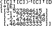
So the best fitting polynomial of degree three is
y = P(x) = 3.523884615 – 1.797352564x – 2.474461538x2 + .4640833333x3
Put this polynomial in \Y2:
\Y2=3.523884615 – 1.797352564X – 2.474461538X2 + .4640833333X3
Activate this equation, and graph it and the 5 points (activate Plot1 to get the 5 points) together. You will see:
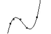
A pretty good fit!
Calculus Index