Cumulative distributions with dice

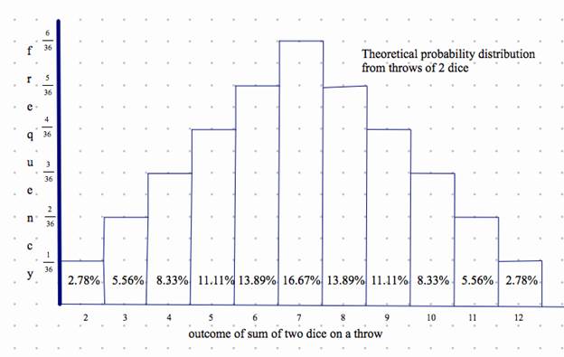
First, a review. Earlier we computed the theoretical frequency distribution for throwing two dice. It looks like this:

Another way to look at the data:

Theoretical probability of the 11 outcomes from tossing two dice

outcome

frequency

(fraction)

1/36

1/18

1/12

1/9

5/36

1/6

5/36

1/9

1/12

1/18

1/36

frequency

(decimal)

.0278

.0556

.0833

.1111

.1389

.1667

.1389

.1111

.0833

.0556

.0278

We discovered that when we randomly toss two dice, we rarely if ever get the theoretical distribution. Instead, we get an empirical distribution that differs from the theoretical one. When we used the program DICETOSS, we saw that most often, if we kept rolling, our whole distribution of observed frequencies came fairly close to the theoretical probabilities.

But now we want to do something different with our calculators. We will program the calculator to draw an empirical bar graph of the CUMULATIVE tosses of two dice, namely, a cumulative distribution of the empirical outcomes.

What is a cumulative distribution? For every number x, you count the total number of data points (here, the number of throws) smaller than or equal to x. For example, if we have the list {2, 4, 6, 2, 3, 5}, and x = 4.5, the number of data points smaller than or equal to x is four (they are 2, 4, 2, and 3).

We can put any set of numbers into list LD. Let’s simulate throwing two dice 200 times. We store the data in list LD. First, store in LD the result of 200 throws of one die:

randInt(1,6,200) → LD

Now let’s add to the list the result of 200 throws of the second die:

randInt(1,6,200)+ LD → LD

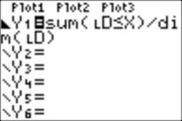
In your calculator, enter

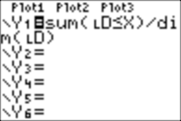
LD≤X returns the value one for any element of the list LD which is less than or equal to X. Y1 computes the frequency, a number between 0 and 1.

To set the window:

Xmin=min(LD)-1

Xmax=max(LD)+1

Ymin=0

Ymax=1

Be sure to set Axes off and Plots off. Now

GRAPH

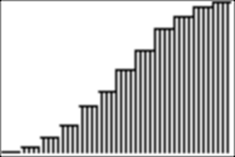
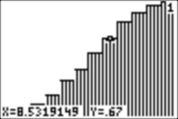
This is what I got. Does yours look something like it?

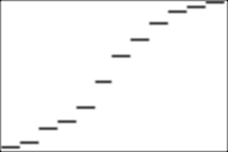
It is called a cumulative distribution.

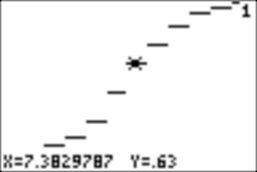
Let’s explore it with TRACE. For example, for X between 7 and 8, TRACE shows the decimal number of throws yielding 2, 3, 4, 5, 6, and 7.

Suppose we want to know the percentage of throws with individual (not cumulative) outcomes of 2, 3, 4, 5, 6, 7, 8, 9, 10, 11, and 12. We do it this way:

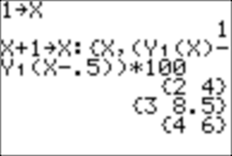
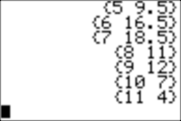
Each time we press enter, we see the outcome and the percentage of throws in list LD

with this outcome.

Now let’s make another empirical cumulative distribution with two dice, as we did earlier:

randInt(1,6,200) → LD

randInt(1,6,200)+ LD → LD

Now in Y=, change Y1 to look as follows:

Then

GRAPH

Here is what I see. What do you see?

You may explore the values using TRACE, as we did above. Here is an example from my run:

How does this empirical distribution compare with the cumulative probability distribution for tossing two dice? Let’s look at the theoretical cumulative distribution numerically:

Theoretical cumulative probability of the 11 outcomes from tossing two dice

outcome

frequency

(fraction)

1/36

1/12

1/6

5/18

5/12

7/12

13/18

5/6

11/12

35/36

frequency

(decimal)

.0278

.0833

.1667

.2778

.4167

.5833

.7222

.8333

.9167

.9722

You can also graph the cumulative probability distribution:

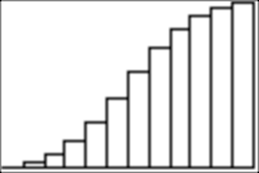
(Can you figure out how to do it? I used StatPlot.)

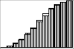
And you can graph the cumulative probability distribution and the empirical frequency distribution on the same screen:

Further, you can investigate both graphs with TRACE:

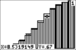
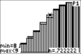
P1 is the cumulative probability distribution and 1 is the empirical frequency distribution.

Your task.

Make an (empirical) cumulative distribution graph on your TI-83/84 for 200 tosses of THREE (or four; you can choose) dice, and show it to the instructor.

How do you set the calculator window? (What is the lowest outcome you can throw with 3 dice? Set Xmin equal to this value minus 1. What is the highest? Set Xmax equal to this value plus 1. Ymin is 0 and Ymax is 1.)

Webpage Maintained by Owen Ramsey
Return