Part 3. A Program, DICETOSS, that
"rolls" two dice in groups of 200 rolls
The program below simulates the roll of two dice in groups of 200 rolls, and plots the frequencies of their outcomes. Using it, we will actually be able "see" how our experimental frequencies "approach" the theoretical probabilities that we studied in Part 1.
Your task is to enter the program into your calculator and set the window, StatPlot, and Format, and to run the program at least for 1000 rolls. Then compare your percentages of different outcomes with your neighbors. Do they look rather similar?
First we present the calculator screen dumps of the program, and then we give an explanation of each line of code. Next we show how to set the window and how to set StatPlot, and we give examples and explanations of the program's output.
Explanation of the "DICETOSS" program
|
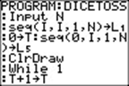
Input N |
N is the length
of lists used in the program. We set
it equal to 12, one more than the 11 outcomes from tossing two dice. |
|
seq(I,I,1,N)→L1 |
List L1 looks as
follows: {1,2,3,4,5,6,7,8,9,10,11,12} |
|
0→T |
T is set at 0
in the beginning. It counts the number of virtual rolls of two dice. |
|
seq (0,I,1,N)→L5 |
The List L5 is filled with 12
zeroes. It is going to keep the counts
of each of the throws 2 through 12. (Its first element will
always be zero, as you cannot roll a one.) |
|
ClrDraw |
The graphing
window is cleared of any drawing. |
|
While 1 |
We start a
loop. The only way to get out of the loop (stop the program is to press ON 1
or ON ENTER. |
|
T+1→T |
Increase the
counter by one. |
|
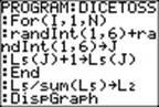
For (I,1,N) |
We are going to
do what follows N times. |
|
randInt(1,6)+ |
Roll the dice
virtually and put the value (which is between 2 and 12) in J. |
|
randInt(1,6)→J |
|
|
L5(J)+1→L5(J) |
Add one to
the Jth element of the list L5. This increases the count of that element
by one. |
|
End |
L5 now contains the individual counts of the
throws from 2 to 12. |
|
L5/sum(L5) →L2 |
The
frequency of each of the 11 outcomes is computed by dividing each count by
the total number of throws, and it is stored in L2. |
|
DispGraph |
Because we have
set the window appropriately, and also set StatPlot1 On, using L1 and L2, a graph will
display in the graph window. It shows graphs of dice throw outcomes 1 through
12 on the X-axis and the frequency of each throw (as a dot) on the Y-axis. |
|
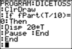
ClrDraw |
The graphs show
sequentially. After appearing briefly, each one is cleared and followed by
the next one. |
|
If fPart(T/10)
= 0 |
If the counter
T is divisible by 10, then display on the home screen 20 times T. This is the
number of rolls that have occurred so far. |
|
Then |
|
|
Disp20*T |
|
|
Pause |
In order to see
the next graphs and count, press ENTER. |
|
End |
|
|
End |
|
To stop the program, press ON 1 or ON ENTER.
To set the window:
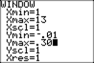
Using StatPlot, set Plot1 On, and set Xlist to be L1, and Ylist to be L2. The tiny open square is a nice choice for showing points.
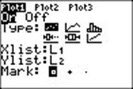
Set Format as follows:
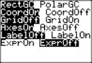
Now we can run the program and explain the output.
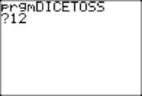
To run the program, select DICETOSS from the Prgm menu. You will see its name on the homescreen together with a ?. Type 12, to indicate that there are 12 possible outcomes. (Actually there are only 11, but we will start our count at 1 to make the screen easier to read.)
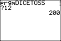
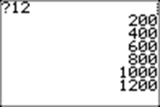
The program simulates the toss of two dice. The first graph that you see shows the results after 20 tosses. The second graph shows the results after 40 tosses. And the tenth graph shows the results after 200 tosses. After every 200 tosses, the program displays the total number of tosses thus far:
You may stop the program at any time by pressing ON 1 or ON ENTER. (When you stop the program, you may not resume it where you left off. But you may start it again from the beginning.) To look at the current graph, press GRAPH.
Here is a graph I got from the program that was stopped after 200 rolls:
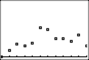 Not
very close to the theoretical distribution!
Not
very close to the theoretical distribution!
So I'll begin again and roll some more.
After 400 rolls,
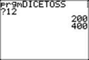
I stopped the program and pressed GRAPH:
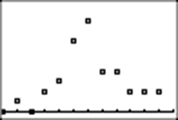
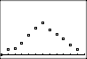
You may continue as long as you want. Here, I stopped the program after 1200 rolls:
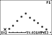
Now I can view the actual percentage of tosses of the throws resulting in the outcomes 2 through 12. I use TRACE.
This means that in 1200 throws, the number 2 came up 3.1% of the time. The theoretical probability for 2 is 1/36, or 2.785%.
If you now look at L1, you will see the empirical frequencies for all tosses, and you may compare each to its theoretical probability.
Return