Part 2. Simulation of tossing a 20-sided (icosahedral) die hundreds of times
A TI-83/84 calculator is needed for this unit.
The program "DISTRIB" below simulates the toss of a 20-sided (icosahedral) die. Of course with 20 possible outcomes (the numbers 1 through 20) equally likely, each has a 5% probability of turning up. So the theoretical distribution will be a constant .05 for each outcome. What we want is to see how close to this distribution we can get by continually rolling the die over and over, in groups of 200 rolls. Each time we can look at the new distribution on the calculator screen. The program also tells us what the difference is in the number of tosses between the highest and lowest totals of tosses, and how far the current highest (or lowest) frequency of tosses is from the probability of .05 or 5%. If we stop the program, we can learn what the 20 actual frequencies are.
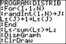
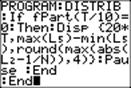
Here is the program that must be entered:
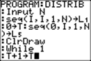
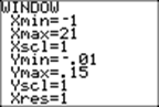
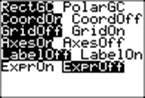
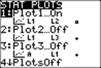
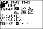
Before you run the program, you need to set the window, set AXES ON in FORMAT, and turn Plot1 on with X variable L1 and Y variable L2:
Here is an explanation of each step in the program. Notice its similarity to the program DICETOSS.
|
Input N |
N is the length
of lists used in the program. We set
it equal to 20, the number of outcomes possible from tossing an icosahedral
die. |
|
seq(I,I,1,N) →L1 |
List L1 looks as
follows: |
|
{1,2,3,4,5,6,7,8,9,10,11,12,13,14,15,16,17,18,19,20} |
|
|
0→T |
T is set
at 0 at the beginning. It counts the
number of virtual rolls of an icosahedral die. |
|
seq (0,I,1,N) →L5 |
The list L5 is filled with 20 zeros. It
is going to keep the counts of each of the throws 1 through 20. |
|
ClrDraw |
The graphing window
is cleared of any drawing. |
|
While 1 |
We start a
loop. The only way to get out of the loop (stop the program) is to press ON 1
or ON 0 |
|
T+1→T |
Increase the
counter by one. |
|
For (I,1,N) |
We are going to
do what follows N times. |
|
randInt(1,N) →J |
Roll the die
virtually and put the value (which is between 1 and 20) in J. |
|
L5(J)+1→L5(J) |
Add one to
the Jth element of the list L5. This increases the count of that element by
one. |
|
End |
L5 now contains the individual counts of the throws from 1 to 20. |
|
L5/sum(L5)→L2 |
The
frequency of each of the 20 outcomes is computed by dividing each count by
the total number of throws. The result
is stored in L2. |
|
DispGraph |
Because we have
set the window appropriately, and also set StatPlot1 On, using L1 and L2, a graph will
display in the graph window. It shows
graphs of dice throw outcomes 1 through 20 on the X-axis and the frequency of
each throw (as a dot) on the Y-axis. |
|
ClrDraw |
The graphs show
sequentially. After appearing briefly, each one is cleared and followed by
the next one. |
|
If fPart(T/10)
= 0 |
Whenever T is
divisible by 10, then the display of graphs is |
|
Then |
interrupted,
and instead, 3 numbers are shown on the home screen: |
|
Disp {20*T,max |
the number of
tosses made so far (a multiple of 200), the difference in number of tosses
between the maximum number and the |
|
(L5)-min(L5),round |
minimum number,
and 20 times the absolute value of the |
|
(max(abs(L2-1/N)), 2)} |
difference of
the biggest or smallest frequency and the probability of .05. |
|
Pause |
In order to see
the next graphs and count, press ENTER. |
|
End |
|
|
End |
|
To stop the program, press ON 1 or ON ENTER.
Then you can look at the 20 frequencies that were obtained in the final graph that was displayed. You do this by pressing TRACE and then the right Gameboy. It will show the x coordinate and the y coordinate, and their values. (Be sure that under FORMAT you have CoordOn turned on; otherwise you will not see the values of the coordinates.)
Here is a run I made. I typed 20 at the ? prompt, because there are 20 outcomes:

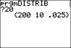
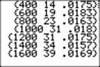
After seeing 10 graphs, {200 10 .025} was displayed on the homescreen.
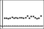
There were 200 throws of one die. This is how the graph looked after 200 throws:
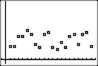
After 200 throws, the largest difference between two outcomes was 10 (the 2nd
number above)..
We can check the graph and see that 5 came up most frequently, 7.5% of the time, and 12 came up least frequently, 2.5% of the time. (Remember that the probability is .05.)
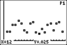
The third number above, .025, is the difference between the current maximum
empirical frequency, .075, and the probability, .05. This number will approach zero as the number
of throws gets huge.
I continued to run the program. Can you explain the three numbers shown after every 200 rolls?
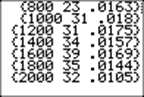
Notice how the third number is getting smaller, while the middle number is not!
What's going on?
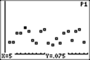
Here's how my graph looked after 2000 tosses:
The smallest frequency was 4.45%, and the largest was 6.05%.
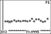
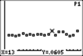
Note that the maximum value, 6.05%, minus the probability, 5%, gives 1.05%, the third number shown.
Your task is to enter the program into your calculator, set the parameters above, and run it for at least 2000 rolls. What do you see?
Return