Part 2.
Simulating a spinner
Here we will enter a program, SPINNER, into our calculators, see that it is used to simulate spins on a dial with sectors like those in Part 1, and run it to collect a lot of simulated data. We want to compute the theoretical frequency of outcomes for the dial, and see if the simulated data, after many spins, approach the theoretical frequency.
Here is the program to be entered:
Explanation of the program
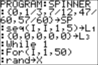
PROGRAM:SPINNER
|
{0,1/3,7/12,47/60,57/60}→SP |
The five sectors on the spinner
dial are 1/3, 1/4, 1/5, 1/6, and 1/20 of the whole circle. Here we do not partition a circle; instead
we partition a segment from 0 to 1 on a number line. The points that
partition the segment are: the 1st point is 0; 2nd point
is 1/3; 3rd point is 1/3+1/4=7/12; 4th point is
7/12+1/5=47/60; 5th point is 47/60+1/6=57/60; and the last point
is 1. The first five points of the partition are put in the list LSP. |
|
seq(I,I,1,5) →L1 |
The numbers 1, 2, 3, 4, and 5 are
put in list L1. They
are the five numbers on the x-axis for our graph, and they represent the five
sectors of the segment. |
|
{0,0,0,0,0}→L3 |
L3 is filled with five zeros at first. Its nth location will store the
number of times (a count) the nth segment is selected by the
random process we program. |
|
While 1 |
We start taking samples. The only
way to interrupt this process is to stop the program by pressing ON 1 or ON
ENTER. |
|
For(I,1,50) |
Fifty more spins are simulated. |
|
rand→X |
rand chooses a number between 0 and 1. Each number is chosen with the same probability; it is rounded to 14 decimal digits, and stored in variable X. |
|
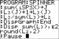
sum(LSP≤X) →J |
LSP≤X returns either 1 or 0 for each number on the list LSP. One is returned if the number is smaller than or equal to X, and 0 is returned when the number is bigger than X. All returned values are added up and stored in variable J. So J counts how many numbers on the list LSP = {0, 1/3, 7/12, 47/60, 57/60} are smaller than or equal to X. As an example, suppose X =
.4. Then 0≤X and 1/3≤X,
but X is smaller than the remaining three numbers. So J = 2, which is the
sector to which X belongs. |
|
L3(J)+1→L3(J) |
L3 contains the number of spins that land in sectors
1, 2, 3, 4, and 5. So 1 is added to
the sector J to which X belongs. |
|
L3/sum(L3) → L2 |
Thinking in terms of a
spinner, L2 keeps
track of the number of times the spinner needle lands in each sector. And L2 records their frequencies. |
|
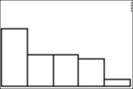
DispGraph |
The graph of the current
frequencies for each of the sectors, one through five, is displayed in a
histogram. |
|
End |
After each 50 simulated spins, a
summary of data is displayed. |
|
Disp sum(L3),E2 round(L2,2) |
The total number of spins up
until now is shown, followed by the percentages of spins, rounded to the
nearest whole percentage, that landed in each of the
five sectors. (E2 is
100.) |
|
Pause |
The user presses ENTER, and the
graph is shown again. |
|
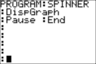
DispGraph |
|
|
Pause |
The next round of fifty spins is
started, and the cycle is repeated. |
|
End |
|
Before you run the program:
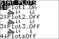
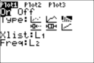
Set the window as follows: And set StatPlot (note the new Type, a histogram):
(Note that Xscl=1.)
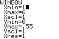
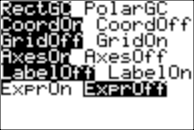
Also be sure to put AxesOn under FORMAT:
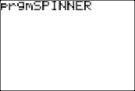
Now to run the program SPINNER, select it and press ENTER:
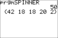
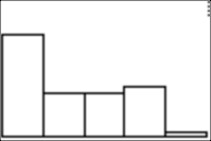
After 50 "spins" (during which you see histograms), you will see the number 50, and the percentages of spins that landed in sectors 1, 2, 3, 4, and 5, rounded to the nearest whole percentage. Here are results when I ran the program. Press ENTER after you see the data, and you will see the current histogram.
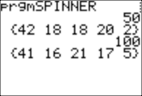
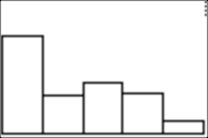
Here are the data and histogram I got after 100 "spins":
And after 150 "spins":
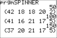
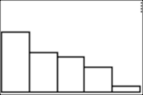
I stopped after 500 "spins", and here are the results:
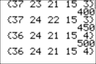
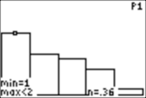
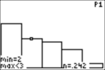
After stopping the program (with ON 0 or ON ENTER), I can use TRACE and see the values for the various outcomes. Here are two examples:
Can you compute the theoretical probabilities for the five outcomes?
Your task is to enter the SPINNER program and run it for at least 500 spins, and to compare your five results to the theoretical probabilities.
Return